Advanced McStas features: SPLIT
Contents
Advanced McStas features: SPLIT
McStas uses the Monte Carlo ray-tracing technique, which allows some tricks on how the physics is sampled as long as the resulting probability distributions match the physics. This is possible as each ray has a weight, corresponding to how much intensity this ray represents. The SPLIT keyword can be used to split a ray into many equal parts, which can be useful if the remaining instrument has many different simulated and random outcomes. In this tutorial we will use the SPLIT keyword on a powder sample, as there are many powder Bragg peaks each ray could select, and splitting the ray samples this more efficiently.
Setting up an example instrument
First we set up an example instrument, this is taken from the basic tutorial and consists of source, guide, monochromator, sample and banana detector.
import mcstasscript as ms
instrument = ms.McStas_instr("python_tutorial", input_path="run_folder",
                                output_path="data_folder/mcstas_SPLIT")
instrument.add_component("Origin", "Progress_bar")

src = instrument.add_component("source", "Source_div")
src.xwidth = 0.1
src.yheight = 0.05
src.focus_aw = 1.2
src.focus_ah = 2.3

wavelength = instrument.add_parameter("wavelength", value=5.0, comment="Wavelength in [Ang]")
src.lambda0 = wavelength
src.dlambda = "0.03*wavelength"

guide = instrument.add_component("guide", "Guide_gravity", AT=[0,0,2], RELATIVE=src)
guide.w1 = 0.05
guide.w2 = 0.05
guide.h1 = 0.05
guide.h2 = 0.05
guide.l = 8.0
guide.m = 3.5
guide.G = -9.82

mono_Q = instrument.add_declare_var("double", "mono_Q", value=1.714) # Q for Ge 311
instrument.add_declare_var("double", "wavevector")
instrument.append_initialize("wavevector = 2.0*PI/wavelength;")

mono_rotation = instrument.add_declare_var("double", "mono_rotation")
instrument.append_initialize("mono_rotation = asin(mono_Q/(2.0*wavevector))*RAD2DEG;")
instrument.append_initialize('printf("monochromator rotation = %g deg\\n", mono_rotation);')

mono = instrument.add_component("mono", "Monochromator_flat")
mono.zwidth = 0.05
mono.yheight = 0.08
mono.Q = mono_Q
mono.set_AT([0, 0, 8.5], RELATIVE=guide)
mono.set_ROTATED([0, mono_rotation, 0], RELATIVE=guide)

beam_direction = instrument.add_component("beam_dir", "Arm", AT_RELATIVE=mono)
beam_direction.set_ROTATED([0, "mono_rotation", 0], RELATIVE="mono")

sample = instrument.add_component("sample", "PowderN", AT=[0,0,1.1], RELATIVE=beam_direction)
sample.radius = 0.015
sample.yheight = 0.05
sample.reflections = '"Na2Ca3Al2F14.laz"'

banana = instrument.add_component("banana", "Monitor_nD", RELATIVE=sample)
banana.xwidth = 2.0
banana.yheight = 0.3
banana.restore_neutron = 1
banana.filename = '"banana.dat"'
banana.options = '"theta limits=[5 175] bins=150, banana"'
Running the simulation
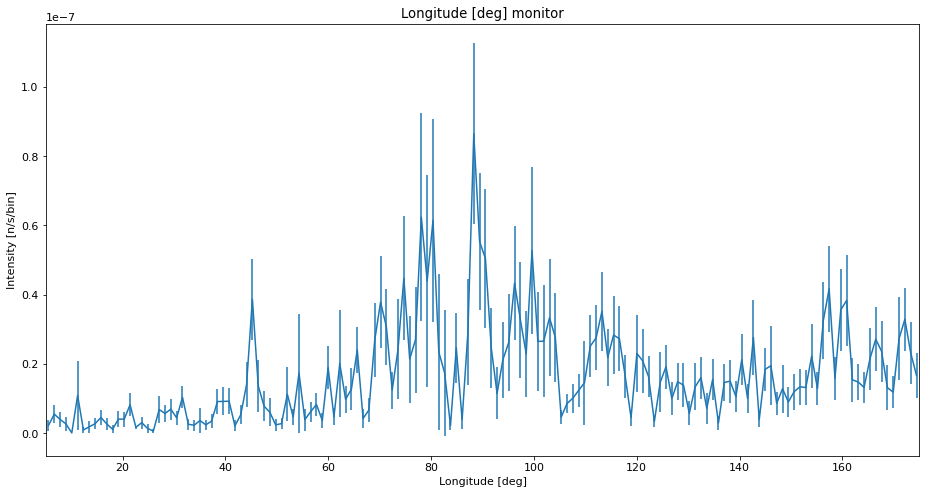
Here we run the simulation with very few neutrons to show problematic sampling.
instrument.settings(ncount=1E6)

instrument.set_parameters(wavelength=2.8)

data_low = instrument.backengine()
INFO: Using directory: "/Users/madsbertelsen/PaNOSC/McStasScript/github/McStasScript/docs/source/tutorial/data_folder/mcstas_SPLIT_3"
INFO: Regenerating c-file: python_tutorial.c
CFLAGS=
      INFO: Recompiling: ./python_tutorial.out
mccode-r.c:2837:3: warning: expression result unused [-Wunused-value]
  *t0;
  ^~~
1 warning generated.
INFO: ===
monochromator rotation = 22.4519 deg
[python_tutorial] Initialize
Opening input file '/Applications/McStas-2.7.1.app/Contents/Resources/mcstas/2.7.1//data/Na2Ca3Al2F14.laz' (Table_Read_Offset)
Table from file 'Na2Ca3Al2F14.laz' (block 1) is 841 x 18 (x=1:20), constant step. interpolation: linear
  '# TITLE *-Na2Ca3Al2F14-[I213] Courbion, G.;Ferey, G.[1988] Standard NAC cal ...'
PowderN: sample: Reading 841 rows from Na2Ca3Al2F14.laz
PowderN: sample: Read 841 reflections from file 'Na2Ca3Al2F14.laz'
PowderN: sample: Vc=1079.1 [Angs] sigma_abs=11.7856 [barn] sigma_inc=13.6704 [barn] reflections=Na2Ca3Al2F14.laz

Save [python_tutorial]
Detector: banana_I=2.50245e-06 banana_ERR=1.15792e-07 banana_N=1445 "banana.dat"

Finally [python_tutorial: /Users/madsbertelsen/PaNOSC/McStasScript/github/McStasScript/docs/source/tutorial/data_folder/mcstas_SPLIT_3]. Time: 0 [s]
PowderN: sample: Info: you may highly improve the computation efficiency by using
    SPLIT 47 COMPONENT sample=PowderN(...)
  in the instrument description python_tutorial.instr.
INFO: Placing instr file copy python_tutorial.instr in dataset /Users/madsbertelsen/PaNOSC/McStasScript/github/McStasScript/docs/source/tutorial/data_folder/mcstas_SPLIT_3
loading system configuration
ms.make_sub_plot(data_low)
Adding the SPLIT keyword
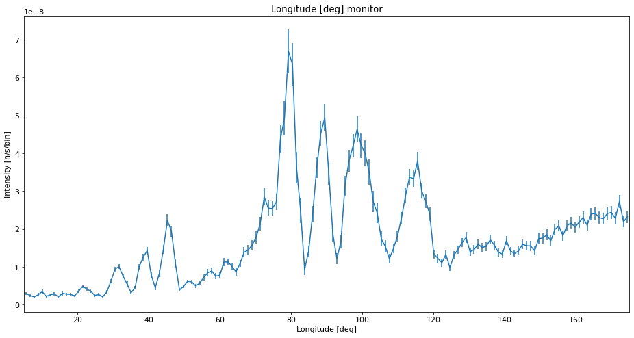
Here we add the SPLIT keyword to the sample, we choose to split each ray into 30.
sample.set_SPLIT(30)
# No need to set settings or parameters as these have not changed
data_reasonable = instrument.backengine()
INFO: Using directory: "/Users/madsbertelsen/PaNOSC/McStasScript/github/McStasScript/docs/source/tutorial/data_folder/mcstas_SPLIT_4"
INFO: Regenerating c-file: python_tutorial.c
Info:    Defining SPLIT from sample=PowderN() to END in instrument python_tutorial
CFLAGS=
      INFO: Recompiling: ./python_tutorial.out
mccode-r.c:2837:3: warning: expression result unused [-Wunused-value]
  *t0;
  ^~~
1 warning generated.
INFO: ===
monochromator rotation = 22.4519 deg
[python_tutorial] Initialize
Opening input file '/Applications/McStas-2.7.1.app/Contents/Resources/mcstas/2.7.1//data/Na2Ca3Al2F14.laz' (Table_Read_Offset)
Table from file 'Na2Ca3Al2F14.laz' (block 1) is 841 x 18 (x=1:20), constant step. interpolation: linear
  '# TITLE *-Na2Ca3Al2F14-[I213] Courbion, G.;Ferey, G.[1988] Standard NAC cal ...'
PowderN: sample: Reading 841 rows from Na2Ca3Al2F14.laz
PowderN: sample: Read 841 reflections from file 'Na2Ca3Al2F14.laz'
PowderN: sample: Vc=1079.1 [Angs] sigma_abs=11.7856 [barn] sigma_inc=13.6704 [barn] reflections=Na2Ca3Al2F14.laz

Save [python_tutorial]
Detector: banana_I=2.60308e-06 banana_ERR=2.14412e-08 banana_N=43854 "banana.dat"

Finally [python_tutorial: /Users/madsbertelsen/PaNOSC/McStasScript/github/McStasScript/docs/source/tutorial/data_folder/mcstas_SPLIT_4]. Time: 1 [s]
PowderN: sample: Info: you may highly improve the computation efficiency by using
    SPLIT 47 COMPONENT sample=PowderN(...)
  in the instrument description python_tutorial.instr.
INFO: Placing instr file copy python_tutorial.instr in dataset /Users/madsbertelsen/PaNOSC/McStasScript/github/McStasScript/docs/source/tutorial/data_folder/mcstas_SPLIT_4
loading system configuration
ms.make_sub_plot(data_reasonable)
Caution on split value
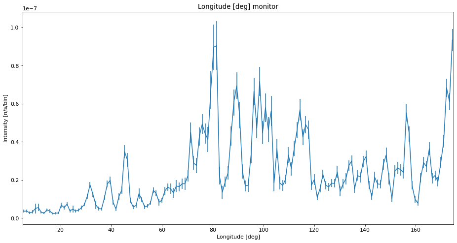
It is however possible to mismanage splitting, mainly by simulating a too few rays and splitting too much. Here we do this on purpose to see how such data would look.
sample.set_SPLIT(10000)

instrument.settings(ncount=1E3) # Change settings to lower ncount, but keep parameters

data_unreasonable = instrument.backengine()
INFO: Using directory: "/Users/madsbertelsen/PaNOSC/McStasScript/github/McStasScript/docs/source/tutorial/data_folder/mcstas_SPLIT_5"
INFO: Regenerating c-file: python_tutorial.c
Info:    Defining SPLIT from sample=PowderN() to END in instrument python_tutorial
CFLAGS=
      INFO: Recompiling: ./python_tutorial.out
mccode-r.c:2837:3: warning: expression result unused [-Wunused-value]
  *t0;
  ^~~
1 warning generated.
INFO: ===
Warning: Number of events 3.21e+06 reaching SPLIT position Component[6] sample=PowderN()
         is probably too low. Increase Ncount.
monochromator rotation = 22.4519 deg
[python_tutorial] Initialize
Opening input file '/Applications/McStas-2.7.1.app/Contents/Resources/mcstas/2.7.1//data/Na2Ca3Al2F14.laz' (Table_Read_Offset)
Table from file 'Na2Ca3Al2F14.laz' (block 1) is 841 x 18 (x=1:20), constant step. interpolation: linear
  '# TITLE *-Na2Ca3Al2F14-[I213] Courbion, G.;Ferey, G.[1988] Standard NAC cal ...'
PowderN: sample: Reading 841 rows from Na2Ca3Al2F14.laz
PowderN: sample: Read 841 reflections from file 'Na2Ca3Al2F14.laz'
PowderN: sample: Vc=1079.1 [Angs] sigma_abs=11.7856 [barn] sigma_inc=13.6704 [barn] reflections=Na2Ca3Al2F14.laz

Save [python_tutorial]
Detector: banana_I=3.61748e-06 banana_ERR=4.48344e-08 banana_N=19572 "banana.dat"

Finally [python_tutorial: /Users/madsbertelsen/PaNOSC/McStasScript/github/McStasScript/docs/source/tutorial/data_folder/mcstas_SPLIT_5]. Time: 0 [s]
INFO: Placing instr file copy python_tutorial.instr in dataset /Users/madsbertelsen/PaNOSC/McStasScript/github/McStasScript/docs/source/tutorial/data_folder/mcstas_SPLIT_5
loading system configuration
ms.make_sub_plot(data_unreasonable)
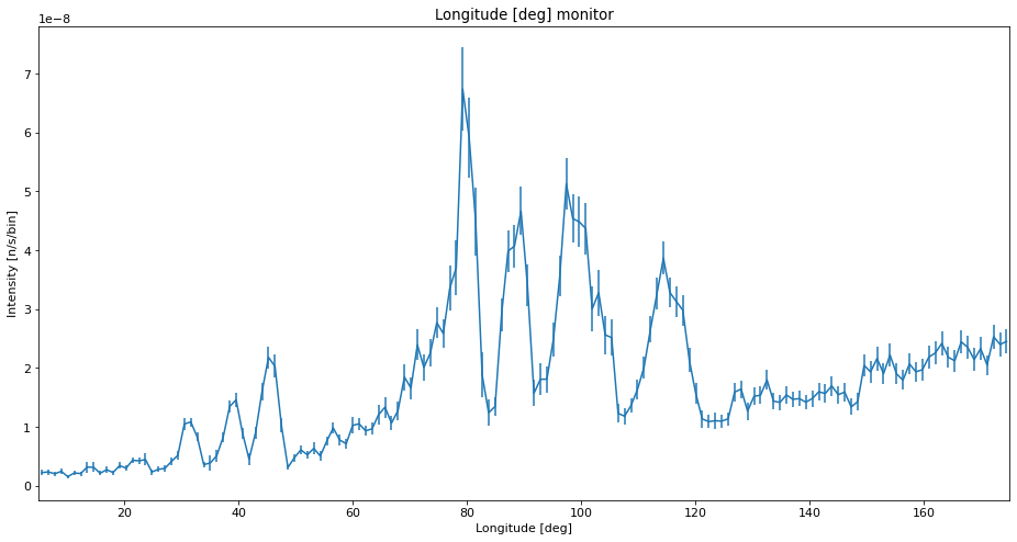
Comparison with high statistics run
We here compare the different runs to a reference. The reference run is set up to have 50 times more rays than the earlier runs with 5E7 instead of 1E6 rays.
sample.set_SPLIT(1)
instrument.settings(ncount=2E7)

data_ref = instrument.backengine()
INFO: Using directory: "/Users/madsbertelsen/PaNOSC/McStasScript/github/McStasScript/docs/source/tutorial/data_folder/mcstas_SPLIT_6"
INFO: Regenerating c-file: python_tutorial.c
Info:    Defining SPLIT from sample=PowderN() to END in instrument python_tutorial
CFLAGS=
      INFO: Recompiling: ./python_tutorial.out
mccode-r.c:2837:3: warning: expression result unused [-Wunused-value]
  *t0;
  ^~~
1 warning generated.
INFO: ===
monochromator rotation = 22.4519 deg
[python_tutorial] Initialize
Opening input file '/Applications/McStas-2.7.1.app/Contents/Resources/mcstas/2.7.1//data/Na2Ca3Al2F14.laz' (Table_Read_Offset)
Table from file 'Na2Ca3Al2F14.laz' (block 1) is 841 x 18 (x=1:20), constant step. interpolation: linear
  '# TITLE *-Na2Ca3Al2F14-[I213] Courbion, G.;Ferey, G.[1988] Standard NAC cal ...'
PowderN: sample: Reading 841 rows from Na2Ca3Al2F14.laz
PowderN: sample: Read 841 reflections from file 'Na2Ca3Al2F14.laz'
PowderN: sample: Vc=1079.1 [Angs] sigma_abs=11.7856 [barn] sigma_inc=13.6704 [barn] reflections=Na2Ca3Al2F14.laz

Save [python_tutorial]
Detector: banana_I=2.59115e-06 banana_ERR=2.62843e-08 banana_N=29429 "banana.dat"

Finally [python_tutorial: /Users/madsbertelsen/PaNOSC/McStasScript/github/McStasScript/docs/source/tutorial/data_folder/mcstas_SPLIT_6]. Time: 10 [s]
PowderN: sample: Info: you may highly improve the computation efficiency by using
    SPLIT 47 COMPONENT sample=PowderN(...)
  in the instrument description python_tutorial.instr.
INFO: Placing instr file copy python_tutorial.instr in dataset /Users/madsbertelsen/PaNOSC/McStasScript/github/McStasScript/docs/source/tutorial/data_folder/mcstas_SPLIT_6
loading system configuration
ms.make_sub_plot(data_ref)
Plotting data on same plot
Here we only have one monitor in each data list, but we still use the name_search function to retrieve the correct data object from each. This avoids the code breaking in case additional monitors are added.
Once we have the objects, we use the xaxis, Intensity and Error attributes to plot the data with matplotlib.
import matplotlib.pyplot as plt
banana_low = ms.name_search("banana", data_low)
banana_reasonable = ms.name_search("banana", data_reasonable)
banana_unreasonable = ms.name_search("banana", data_unreasonable)
banana_ref = ms.name_search("banana", data_ref)

plt.figure(figsize=(14,6))
plt.errorbar(banana_low.xaxis, banana_low.Intensity, yerr=banana_low.Error, fmt="r")
plt.errorbar(banana_ref.xaxis, banana_ref.Intensity, yerr=banana_ref.Error, fmt="b")
plt.xlabel("2Theta [deg]")
plt.ylabel("Intensity [n/s]")
plt.legend(["Low statistics", "High statistics reference"])

plt.figure(figsize=(14,6))
plt.errorbar(banana_reasonable.xaxis, banana_reasonable.Intensity,
             yerr=banana_reasonable.Error, fmt="r")
plt.errorbar(banana_ref.xaxis, banana_ref.Intensity, yerr=banana_ref.Error, fmt="b")
plt.xlabel("2Theta [deg]")
plt.ylabel("Intensity [n/s]")
plt.legend(["Low statistics with SPLIT", "High statistics reference"])

plt.figure(figsize=(14,6))
plt.errorbar(banana_unreasonable.xaxis, banana_unreasonable.Intensity,
             yerr=banana_unreasonable.Error, fmt="r")
plt.errorbar(banana_ref.xaxis, banana_ref.Intensity, yerr=banana_ref.Error, fmt="b")
plt.xlabel("2Theta [deg]")
plt.ylabel("Intensity [n/s]")
l = plt.legend(["Very low statistics with unreasonable SPLIT", "High statistics reference"])
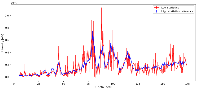
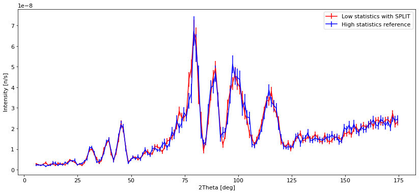
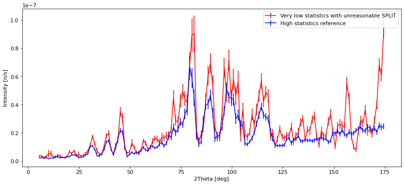
Interpretation of the data
We see that with low statistics, the data quality is so bad that noise can be mistaken for peaks. Using SPLIT improves the situation a lot, and the data is very similar to the high statistics reference which takes longer to compute. The situation with a low number of simulated rays and very high SPLIT have some erratic behavior, showing some very different peak intensities than the reference, and some peaks that shouldn’t be there at all.